Cost budgeting

Introduction

Cost budgeting involves aggregating the estimated costs of individual schedule activities or work packages to establish a total cost baseline for measuring project performance.

Although the project manager may be able to calculate a total budget based on assigned resources early in the project, it is important to determine when money will be spent during the project life cycle. The timing of these planned costs will require other parts of the organization to coordinate so that the costs can be properly funded and paid for on a timely basis.

Cost budgeting occurs after cost estimating. Many projects start with a total budget before the specifics of a project are defined, but in many cases, these preset budgets may be reconsidered after cost estimation occurs. Cost budgets are also frequently adjusted in response to other project management processes, illustrating the iterative nature of the project management process.

On some projects of smaller scope, cost estimating and cost budgeting are so tightly linked that they are viewed as a single process that can be performed by a single person over a relatively short period of time. There are distinct processes being applied, however, as the inputs, tools and techniques and outputs for each are different. Early scope definition is critical to both processes, as the ability to influence project cost is greatest at the early stages of the project.

Cost budgeting involves summing the estimated costs of the work activities at the work package level or higher, depending on the needs of the project and the policies of the performing organization. If bottom-up estimation was used to estimate activity costs, a time-phased budget at the activity level can be produced by allocating the activities' costs to the time periods in which the project schedule says the activities will take place. Rolling activity costs up to the work package level is then straightforward.

Baseline spend curve

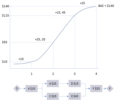
The baseline S-curve shows the total planned cumulative expenditure, period by period throughout the duration of the project. At the planned end date of the project, the cumulative cost reaches the full budget amount, known as budget at completion (BAC).

In the simplified example below, a project consisting of 6 tasks is shown. Tasks are labeled A through F, and each is associated with a cost. The network diagram at the bottom illustrates the dependencies among the tasks.

• At the end of time period 1, task A has completed, so the cost expended after period 1 is $10.

• At the end of time period 2, tasks B and C have also completed, so the cost expended after period 2 is ($10 + $25 + $20) = $55.

• At the end of period 3, tasks D and E have also completed, so the cost expended after period 3 is ($55 + $15 + $45) = $115.

• At the end of period 4, task F has completed, so the cost expended after period 4, the end of the project, is ($115 + $25) = $140. This is the budget at completion, as it represents the planned cumulative costs to be expended on the project.

 

 

As project performance information is periodically collected, the comparison of actual costs to the planned budget baseline will provide vital information concerning the health of the project. Summarizing both values using this cumulative cost graph technique provides a quick visual indicator of any problems in managing project costs. This will be discussed further in the context of the Cost Control process.

Cost budgeting process inputs

• Project scope statement
  

• The project scope statement describes any funding constraints, such as required fiscal year boundaries and other funding cycles that limit the acquisition and expenditure of funds.

• Work breakdown structure (WBS)
  

• The WBS provides the relationship between project components and project deliverables. This provides the structure for the aggregation of costs used for budgeting, monitoring, and control.

• WBS dictionary
  

• The WBS dictionary, the companion document to the WBS, contains the details for each component, includes a code or account identifier, statement of work, responsible organization, and a list of milestones. Other information can include a list of associated schedule activities, resources required, and an estimate of cost.

• Activity cost estimates
  

• The activity cost estimates represent the cost data that will form the basis of the amounts in the cost budget.

• Supporting detail for activity cost estimates
  

• The supporting detail for the activity cost estimate describes how the estimates were formed and provides the basis for determining the accuracy of the estimates. The degree of uncertainty in the estimates will be used to gauge how much additional funding may be necessary to cover estimating errors.

• Project schedule
  

• The project schedule includes the planned start and finish dates for the activities, work packages, planning packages, and control accounts. These dates are used to allocate estimated costs to the calendar periods in which they are planned to occur.

• Resource calendars
  

• The resource calendar shows holidays and the availability of specific resources. It defines calendar periods within an activity's duration during which costs can or cannot occur, due to the availability of key resources. This prevents funding requests and cost expenditures from being scheduled on holidays or during the absence of the authorizing stakeholder or project manager.

• Contract
  

• A contract can be a complex document or a simple purchase order. Regardless of the format, a contract is a binding legal agreement. The contract supplies information about what products, services, or results have been purchased, along with their costs.

• Cost management plan
  

• The cost management plan, a component of the project management plan, defines how cost budgeting will be carried out.

 

Cost budgeting process tools

Cost aggregation

To make monitoring and controlling costs easier, schedule activity cost estimates are aggregated by the work packages that comprise the WBS. The work package cost estimates can then be aggregated at higher levels of the WBS, if needed, to reach the summary level needed for the performing organization's financial control method.

 

 

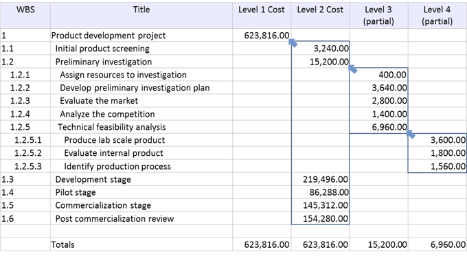
The above example illustrates the concept of cost aggregation. The first column shows the WBS number for the work package that the activity will produce. Here, the WBS numbering system uses an outline scheme to indicate which components fit into others.

The names of the schedule activities and their summary elements appear in the second column.

The use of the bottom-up estimating technique has resulted in a cost estimate for each Level 4 (lowest-level) work package. In the example, only the work packages 1.2.5.1 through 1.2.5.3 are shown at this level.

The sum of these three Level 4 work packages is $6,960. This total amount is considered the aggregated cost for these work packages and is shown as the estimate for the Level 3 control account 1.2.5, "Technical feasibility analysis."

The values of each Level 3 control account are also aggregated. In this case, only the control accounts 1.2.1 through 1.2.5 are shown. They aggregate to $15,200, which is shown as the Level 2 cost estimate for control account 1.2, "Preliminary investigation stage."

Finally, while not explicitly illustrated on the diagram, the aggregated amounts for each Level 2 control account are summed or aggregated to produce the total project estimate, shown as the Level 1 Cost of $623,816 for the Product development project.

The process that the project management team and sponsor use for monitoring and controlling the costs will generally specify a level of detail at which costs should be budgeted and tracked, and variances reported. This makes it easier to locate where significant variances are occurring without reviewing potentially large amounts of insignificant detail, and provides the most control for the minimum effort.

The level of aggregation may also vary from one part of the project's work to another, if some activities run more significant risks of cost overruns than others. In the example above, the Technical feasibility analysis (WBS 1.2.5) costs are being budgeted at the detail level of the work package, but the Initial product screening stage (WBS 1.1) was budgeted only at the highest ("stage") level. The risk of a significant overrun in the Initial product screening stage was deemed too low to break down the costs further.

 

Cost budgeting techniques

Parametric estimating

When specific schedule activities have not been defined and estimated, parametric estimating can be applied to the planning components to provide a high-level budget for the affected work. This will generally be necessary when the project is in the conceptual stage of development and the details of the work are not known. It is also true in rolling wave planning for later phases. In this case, the later phases are not planned in detail, pending the availability of missing information. For the next phase, the necessary detail will be produced only as an outcome of the current work.

In these situations, using parametric estimating at the phase or other planning component level can set the budget. For parametric estimating to be most effective, the following should be considered:

• The model that is used should be based on accurate historical information;
• The model should work for different sizes of projects (in other words, the model should be scalable); and
• The parameters used in the model should be quantifiable.

Reserve analysis sets aside reserves to be used for unplanned changes. The changes might be due to anticipated risks and thus involve the cost of the contingency plan, or they might be due to an anticipated rate of errors and rework ("known unknowns", or contingency reserves). On the other hand, they might be the result of unexpected events that require workarounds, and for which no contingency plan exists ("unknown unknowns", or management reserves).

Management reserves are not part of the project cost baseline, but they are included in the budget for the project. Cost budget reserves are discussed in more detail in a subsequent section.

Funding limit reconciliation

The timing of funds and planned costs for projects must solve two problems: solvency and fiscal timing.

For a project to be solvent, funds must always be available to meet planned costs. This means that, for any given period, the level of available funds will always be slightly higher than the amount required by the total time-phased budget baseline. The principle is the same as the funding requirement for a personal bank checking account.

Funds must also match the timing of the planned costs within the organization's fiscal cycles. This is the case even if the planned costs shift due to schedule changes. Funds are authorized for disbursement to the project in cycles that are set by the customer or organization to follow their fiscal cycles. The funds can then be spent only for work performed in the same fiscal cycle.

For example: Funds for work in a company's fiscal year 2016 will be disbursed shortly before the start of the fiscal year. They can then be used only to pay for invoices that relate to work that was completed in the same fiscal year.

Unused funds expire at the end of the fiscal year, and, conversely, if there are overruns, they must be accommodated through additional funds disbursed in the same fiscal year.

Because work may accelerate or slip across fiscal cycle boundaries, every time the schedule changes, the funds made available must be reconciled with the actual budgeted costs. When the disbursed funds cannot cover the additional costs, or when there will be excess funds in one cycle and a shortage in the next, the usual technique is to shift other portions of the work between the fiscal periods. This maneuver reduces the overrun or consumes the excess. This is done by imposing date constraints on some work packages, schedule milestones, or WBS components in the project schedule.

Reconciling the funding limit is normally performed by the finance function within the organization. It is unusual to simply request changes in the fund disbursement schedule, because the planned expenditures on a given project must be balanced with the total available cash flow in the organization, taking into account the priorities of other projects and business operations. If funding were constantly being shifted, managing the cash flow would become extremely difficult.

The cost budgeting process produces the following outputs:

• Cost baseline;
• Project funding requirements;
• Updates to the cost management plan; and
• Requested changes.

Cost baseline

The primary goal of the cost budgeting process is to determine the cost baseline. Once the cost budget is approved, it becomes the cost baseline. The cost baseline will be used to measure and monitor cost performance on the project. As noted earlier, the cost baseline is developed by summing estimated costs by period and is usually displayed in the form of an S-curve.

Some projects may have multiple cost or resource baselines to measure different aspects of project performance. For example, internal labor costs may be tracked separately from external costs of contractors or from total labor hours.

Project funding requirements

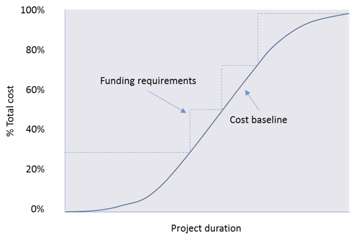
Funding requirements are derived from the cost baseline and must exceed the cost baseline in every period by an amount that will cover expenditures associated with both early progress and cost overruns. Funding occurs in incremental amounts. Each increment must be sufficient to cover all expenditures in every period between the posting of the first increment and the posting of the next increment.

The diagram below shows the comparison of the funding levels to the cost baseline results. The funding requirements are always higher than the project cost baseline's S-curve, as the total funds include the cost baseline plus the management contingency reserve. Some portion of the management contingency reserve can be included incrementally in each funding increment or funded when needed, depending on organizational policies.

 

 

Keeping the budget up to date

The cost management plan is updated with approved change requests that resulted from the cost budgeting process if those approved changes impact the management of costs.

Requested Changes

When budgets are allocated to fit within constraints, some control accounts may not have funding that is sufficient to accomplish the required scope. A change request is then necessary to request additional funding, reduce the scope, or perhaps adjust other planning documentation such as the risk response plan. Requested changes are processed for review and distribution through an integrated change control process.

Cost budget reserves

As noted previously, reserves analysis is a Cost Budgeting technique used to identify the areas in need of reserves. Typically, budget allocations provide challenges to individual control accounts. In order to mitigate the risk of insufficient funds, it is appropriate to establish a cost reserve.

Types of reserves

• Contingency reserve
  

• A contingency reserve is an amount set aside to account for known risks or uncertainties identified in the estimates. For example, during the estimating process, an estimate for the likely amount may have been established, but a more pessimistic or conservative amount was considered plausible. The budgeting strategy in this case could be to set the budget at the lower amount and to reserve the difference in a special contingency amount. The project manager's strategy will be to actively monitor the planning component that the reserve covers so that the costs are controlled within the lower amount. The reserve is available as a safety net, but can be released if it is not required.

• These contingency reserves are estimated costs to be used at the discretion of the project manager to deal with estimating errors and with risk events that have been identified in the risk register (the catalogue of identified project risks).

• These risk events are called "known unknowns," because although their size cannot be predicted with certainty and they may not occur at all, their causes are familiar, and their impacts tend to follow similar patterns on similar projects. Their risk response plans and associated contingency reserves are part of the project scope, schedule, and cost baselines.

• Management Reserve
  

• In some cases large, unexpected risks that impact the project budget may materialize. These risks are referred to as "unknown unknowns," because their size, cause, and likelihood are all impossible to predict. An example might be a labor strike in the middle of a long construction project.

• In the case of these unknown unknowns, the project manager may need to draw on additional funding that was not part of the budget. For this reason, the sponsor's management may agree to set aside an additional reserve called the management reserve that may be drawn upon to deal with unplanned events, but only with their specific approval.

• Since such events by definition cannot be foreseen, the project management team may perform a reserve analysis based on the experiences of prior, similar projects. This management reserve is excluded from the cost budget, but is part of the total funding request.

• Appropriate use of reserves
  

• Reserves should not be used to accommodate scope changes. Any addition to project scope must be formally initiated with a change request, and corresponding adjustments to budget and schedule baselines must be negotiated.
  

• Mature project management cultures understand the benefits of identifying uncertainties and establishing a reserve mechanism to actively manage risks and uncertainties. Less mature organizations may treat reserves with skepticism and may automatically disallow any budget category identified as a contingency. Often these same organizations wonder why they are constantly struggling with projects that cannot be completed within their budgets.
  

• The uncertainty of cost estimates and the occurrence of risk events are unavoidable. Because they are not certain, they should not be factored into the base estimates for the project work. To shield the project from the turbulence that would result when these estimating errors and risk events surface, the project management team should put in place the appropriate reserves, and carefully control their use to meet only the intended purposes.

Reserve analysis and estimating methods

To develop and establish the appropriate cost reserves, the project management team must use the reserve analysis technique, defined earlier.

The method that should be used to establish cost reserves for a planning component or work package depends on the type of estimating method that was originally used to establish the budget. Recall the estimating methods previously discussed:

• Analogous (also known as Top-down);
• Parametric;
• Bottom-up.

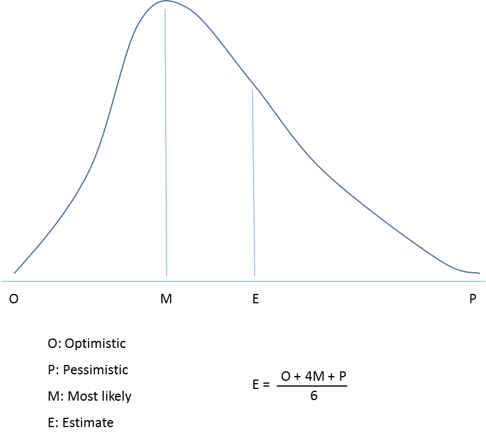
In addition, range estimating, also known as three-point estimating, may be used. Three-point estimates for activity durations are based on three types of estimates:

• Most likely: The duration of the schedule activity, given the resources likely to be assigned, realistic expectations of availability for the schedule activity, dependencies on other participants, and interruptions;
• Optimistic: The activity duration is based on a best-case scenario of what is described in the most likely estimate; and
• Pessimistic: The activity duration is based on a worst-case scenario of what is described in the most likely estimate.

An activity duration estimate can be constructed by using an average of the three estimated durations. That average will often provide a more accurate activity duration estimate than the single-point, most likely estimate. In the diagram below, a weighted average has been used to determine the estimate, as more weight has been given to the most likely estimate.

 

 

The following table describes how one might establish the cost reserve based on the estimating method applied.

 

Estimating method	Establishing the reserve
Analogous/Top-down estimating	Evaluate the degree to which the historical project(s) used as the basis for the analogous estimate differ in terms of complexity, resource types, and optional elements of scope. Establish a general contingency percentage based on the accuracy level predicted of the estimate, e.g., 30%, and apply that percentage contingency to each control account.
Parametric estimating	Evaluate the sensitivity of the parametric measures and devise a contingency. For example, for material, if measurements were accurate within 10%, use a 10% contingency. Also, consider adding a contingency for scrap or wasted material, or expected product defect rates.
Bottom-up estimating	Collect the contingencies estimated for specific activities or work packages into a common contingency account.
Range, or Three-point, estimating	Establish a contingency based on the difference between the "most likely" estimate and three-point estimate, as illustrated below.

 

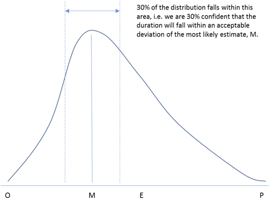
The diagrams below illustrate the calculation of contingency for three-point estimates. It is important to establish a reserve proportionate to the amount of uncertainly represented by the range of the estimate.

In the diagram below, using statistical analysis one can determine that the confidence of achieving M is about 30%, which is not high.

 

 

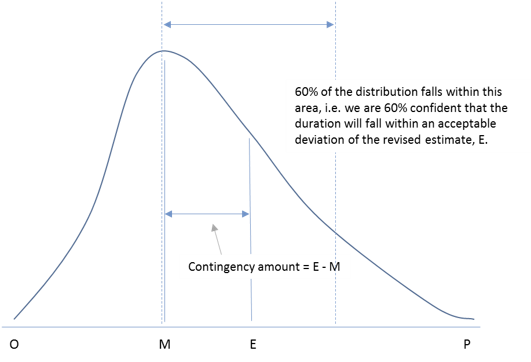
By adding a reserve represented by the difference between the three-point estimate and the most-likely estimate (E M), the confidence of success is closer to 60%.

 

 

Confidence intervals are a statistical concept that is beyond the scope of this article. However, given an estimate that was generated using the three-point estimating technique, a project manager should be able to determine an appropriate contingency amount proportionate to the amount of uncertainty represented by the range of the estimate.

For example, if the supporting detail of a work package estimate noted that the Three-Point Estimating technique was used with the optimistic estimate being $2,500, the most likely estimate being $3,000, and the pessimistic estimate being $5,000, then the project manager would calculate an estimate E = (O + 4M + P) / 6, or [$2,500 + (4 x $3,000) + $5,000] / 6 = $3,250. The project manager could then establish a reserve amount based upon the formula of E - M, or $250 ($3,250 - $3,000).

Similarly if the supporting detail of a work package estimate noted that the Three-Point Estimating technique was used with the optimistic estimate being $100, the most likely estimate being $1,000, and the pessimistic estimate being $10,000, then the project manager would calculate an estimate E = [$100 + (4 x $1,000) + $10,000] / 6 = $2,350. The project manager could establish a reserve amount based upon the formula of E - M, or $1,350 ($2,350 - $1,000).

Note that in the two examples above, the amount of the reserve changes to reflect the amount of uncertainty represented by the range of the estimate. In the second example, there is a greater variance between the optimistic, most likely, and pessimistic estimates, so the reserve amount is greater to reflect this uncertainty.

 

 

Thanks to Ignacio Manzanera for providing this book